The ANOVA : a quick overview
This article explores the principles underlying the Analysis of Variance (ANOVA) as well as the workflow to implement it.
When to perform an Analysis of Variance
The Analysis of Variance (ANOVA) is used to model a continuous response variable as a function of one (or more) categorical explanatory variable(s).
ANOVA models are usually referred to as:
• One-way ANOVA, when the model considers one categorical explanatory variable that has more than two levels
• Two-way ANOVA, when the model considers two categorical explanatory variables that have more than two levels
• and so on.
Actually, the term Analysis of Variance can be source of misunderstanding since this statistical technique is an extension of the independent t-test (used for comparing means in two different groups, i.e. when the categorical explanatory variable that has just two levels). Therefore, like the t-test, the aim of ANOVA is to analyze means among groups and not variance.
The ANOVA is usually employed in the context of experiments to highlight the impact of a factor (or multiple factors) on a quantitative variable (e.g. in case of medical treatments to assess if some quantitative indicator of recovery is significantly different among groups of patients treated with different drugs).
In those case, the ANOVA allows to test if there are differences when comparing the means of the target variable across different groups identified by a level of the factor of interest.
The Underlying Principle
If we want to check if a given factor plays or not a role in determining the value of a quantitative variable, we can perform a one-way ANOVA. This technique allows to assess if the means of the groups identified by the level of the factor under investigation are significantly different from each other.
Considering a factor having k levels, the overall null hypothesis for the ANOVA is
The alternative hypothesis is that “at least one of the k population means differs from all of the others”.
The statistic which measures if the means of different groups are significantly different or not is called the F-Ratio and its mathematical expression is
The higher the F-Ratio value, (and the lower the related p-value) the higher the evidence that the null hypothesis has to be rejected.
From the expression above we can see that the logic underlying the ANOVA is to compare the inter-group variability (i.e. the variability of the target variable within each group) and the intra-group variability (i.e. the variability of the target variable among groups).
Model Assumptions
- Independence of observations (this assumption has to be validated at the experiment-design stage)
- Homoskedasticity of residuals
- Normal distribution of residuals
Steps to implement ANOVA
1. EDA: Side-by-side Boxplots
2. ANOVA test
3. Multiple pairwise-comparison and Results Interpretation
4. Model Validation
1. EDA: Side-by-side Boxplots
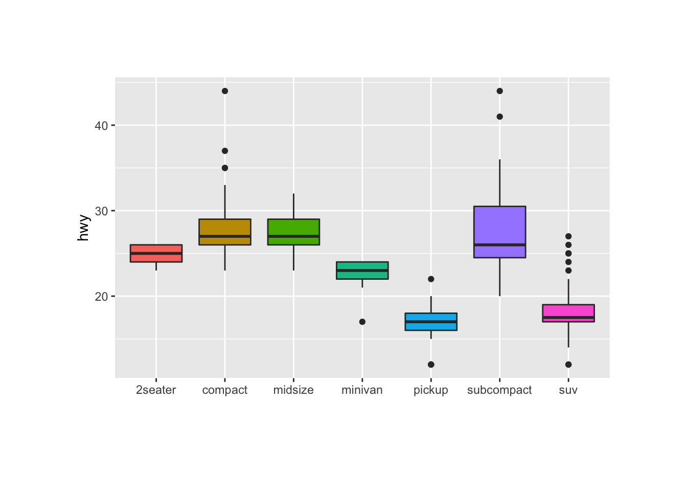
The first step is to visualize how the target variable is distributed across the groups identified by each level of the categorical variable.
The appropriate plot for that is a box-plot which resumes a lot of information about the target variable distribution and allow to formulate some initial hypothesis.

2. ANOVA test
After inspecting the data and formulating the hypothesis,an ANOVA test is performed in order to assess if there is any significant difference between the average value of the target variable across the groups.
Statistical software display ANOVA results in a table as follows:

The ANOVA table includes:
- The factor(s) to be examined (which represents the source of variation). In this case, it is identified by the variable ‘Trt’.
- Sum of Squares (SS) for each source of variation
- Mean Square, i.e. the sum of squares for each factor divided by its associated degrees of freedom (Df)
- F-statistic: built as the mean square of the factor divided by the mean square of the residuals
- Prob > F: the p-value
In order to evaluate the results of the test we need to consider the p-value.
The smaller the p-value is, the higher the evidence that the mean values across groups are different
At the opposite, we have to evaluate the null hypothesis that all the means are the same true
3. Multiple pairwise-comparison and Results Interpretation
An ANOVA is a global test which does not explain where is located the source of the difference, i.e. which mean or means differs from the other.
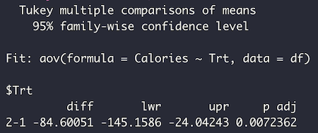
In order to answer this question, we have to use the Tukey multiple-pairwise comparison t-test.

The output gives the difference in means, confidence levels and the adjusted p-values for all possible pairs.
In the example above, the factor of interest has only 2 levels (trt1 and trt2) and the p-value shows that there is a significant between-group difference for the two treatments.
4. Model Validation
The final step is to assess whether ANOVA Assumptions are validated or not. This can be achieved by analyzing residuals’ distribution.
Further details about assessing assumptions validation can be found here
