Linear Models’ Assumptions
The aim of this article is to present regression assumptions as well as how to visually check if a data set validate those assumptions (both visually and using statistical tests).
Focus on Linear Regression
Linear regression models allow to predict a continuous outcome as a function of one or multiple continuous variables.
Linear Regression models are divided in:
- Univariate Linear Regression (or Simple Linear Regression), if the model deals with one input (referred to as independent or predictor variable) and one output variable (referred to as dependent or response variable)
- Multivariate Linear Regression if the model deals with more than one input variable
The aim of linear regression is to establish a function that explains the relationship between the predictor variable(s) and the response variable.
This mathematical equation can be generalized as a linear equation in the following form:
where
is the vector of independent variables
is the response variable
is the predicted value you get when
is a vector of values explaining the change in
when each variable in
change by 1 unit
- ε is the error term, or residual, i.e. the part of
the regression model is unable to explain.
Residuals are defined for each observation as the difference between the actual and predicted values
Regression Diagnostic
Regression is a parametric approach. ‘Parametric’ means it makes some restrictive assumptions about data for the purpose of analysis.
Once these assumptions get violated, regression makes biased, erratic predictions (in those cases, a non-linear model is the only solution) .
Therefore, to be sure to build an accurate regression model, it’s essential to validate these assumptions.
Linear Model’s Assumptions
The five standard assumptions for regression analysis are:
- Linear relationship assumption
This assumption implies that there should be a linear and additive relationship between the response variables and the predictor(s).
A linear relationship means that change in response y due to one unit change in X is constant
An additive relationship suggests that the effect of X on y is independent of other variables
When this assumption is validated, we are sure that our estimator and predictions are unbiased. justify;”}
- Absence of Multicollinearity, i.e. the independent variables should be not correlated.
- Absence of Autocorrelation, i.e. residuals should be not correlated.
If this assumption is not satisfied, our estimator will suffer from high variance.
- Homoskedasticity, i.e. residuals must have constant variance.
When this assumption is not validated, we talk about heteroskedasticity.
Generally, non-constant variance arises in presence of outliers or extreme leverage values. These values get too much weight, hence disproportionately influences the model’s performance. When this phenomenon occurs, the confidence interval for out of sample prediction tends to be unrealistically wide or narrow.
- Normality of Residuals. The error terms should have a normal distribution, with mean 0.
How would you check (validate) if a data set follows all regression assumptions?
The most intuitive tools to check it are the Residuals Plots (explained below) along with some statistical test.
Visually check for assumptions validation.
- Linearity
To check the linearity assumption is enough to plot the predictors versus response variable.
-
Absence of Multicollinearity.
To check if there is multicollinearity, we can compute correlation cofficients. Predictors that are multicollinear have high correlation coefficient (0.80 or higher).
Another way is to perform a Principal Component Analysis and analyze the variable’s plot looking for variables which are correlated each other. -
Absence of Autocorrelation and Homoskedasticity
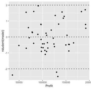
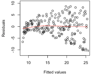
To check for those assumption, the standardized residual plot against fitted values (predicted values) is used.
Residual plots are a valuable source of information to check for a large part of assumptions. The logic is: if the selected independent variables describe the relationship so thoroughly, then only random error will remain. Non-random patterns in residuals suggest that the explication power of the model can be further improved.
When those assumptions are validated, residuals are randomly distributed as in the plot below

Any noticeable pattern in such plots indicates violation of those assumptions. The most typical pattern for nonconstant variance is a plot of residuals versus fits with a pattern that resembles a sideways cone as in the plot below

- Normality of Residuals
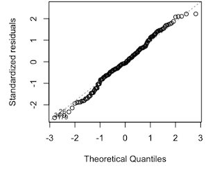
Checking if residuals follow a normal distribution, by examining a normal probability plot of standardized residuals. A straight-line pattern for a normal probability plot indicates that the assumption of normality is validated as in the plot below

When the data is not normally distributed a non-linear transformation (e.g., log-transformation) might fix this issue.
Statistical test for assumptions validation.
- Linearity
Harvey-Collier test, which is a t- test for 0 mean (it tests whether recursive residuals have mean 0 - which they should under the null hypothesis of linearity)
- Absence of Autocorrelation
Durbin-Watson test, which tests the null hypothesis that the residuals are not linearly auto-correlated.
The statistical test can assume values between 0 and 4. As a rule of thumb values between 1.5 and 2.5 show that there is no auto-correlation in the data.
- Homoskedasticity
Goldfeld-Quandt test can also be used to test for heteroscedasticity. The test splits the data into two groups and tests to see if the variances of the residuals are similar across the groups.
- Normality of Residuals
Shapiro-Wilk test
