Inside the Random Forest Black-Box

Random Forest is a non-parametric supervised learning algorithm which belongs to the category of ensemble learning algorithms, meaning it makes prediction by combining the results from many models (i.e. individual decision trees).
The main idea behind the ensemble learning is that combining individual weak predictions together leads to more robust overall prediction.
How Random Forest are built
The individual decision trees built by the Random Forest algorithm are constructed independently using the bagging technique (where bagging stands for Bootstrap Aggregating).
Through bagging, the Random Forest algorithm randomly samples training data points when building trees and randomly selected subsets of features which will be used when splitting nodes (this is the bootstrap part of the bagging technique).
It means that each individual decision tree in the forest considers a random subset of features when performing splits and it is trained on a randomly sampled subset of the data (where sampling is done with replacement, meaning that there could be repeated values in each of the newly created subsets).
Finally, predictions are made by aggregating the predictions of each decision tree (this is the aggregation part of the bagging technique):
- In case of a regression problem, the prediction for a new record is calculated by taking the average of all values predicted by all the individual decision tree;
- in case of a classification problem, the new record is assigned to the category which has been the most frequent predicted by each individual tree.
Bagging is the main reason why Random Forests perform better than individual decision trees.
Indeed, it allows to:
1. Overcome the problem of overfitting.
2. Decrease the overall variance of the model. By training each tree on different samples, although each tree might have high variance with respect to its particular set of the training data, overall, the entire forest will have lower variance.
3. Remove trees correlation, since individual trees are trained on randomly sampled subset if data and features.
To recap, given a dataset containing M observations and K features, the steps taken to implement random forest can be generalized as follows:
• Randomly selection (with replacement) of a subset of m data points.
• Randomly selection (with replacement) of a subset of k features. Whatever feature gives the best split is used to split the node iteratively
• The above steps are repeated until the desired number of tree n (a hyperparameter of the model) is reached. The prediction is given based on the aggregation of all the individual predictions from the n trees
Hyperparameters
In order to optimize model’s performance (i.e. to increase its predictive power or to improve its computational efficiency), there are several hyperparameters that should be considered when training a Random Forest algorithm.
With reference to the Python sklearn built-in RandomForest algorithm, the main parameters to consider are:
• n_estimators: The number of trees in the forest.
A good rule of thumb is to start with 10 times the number of features.
Usually the higher the number of trees the better the model will learn the data. However, adding a lot of trees can affect computational speed without any improvement in model accuracy.
• max_depth: The maximum depth of the tree.
By default, it is None, meaning that the nodes are expanded until all leaves are pure.
The deeper the tree, the more information it is able to learn about the data. However, increasing depth of the tree above a certain level makes the model prone to overfitting.
• max_features: The number of features to consider when looking for the best split in each individual tree.
There are several options available to set this parameter (for further details check the documentation)
• min_samples_leaf: The minimum number of data points allowed in the end node of each decision tree.
Hyperparameters in action
A practical illustration of how model hyperparameters can affect performance is provided by the the following example.
Given different features which are considered important during the application for Master’s Programs, we want to build a model to predict a student’s chances of admission for a particular university .
The dataset is available here whereas the full code is available here.
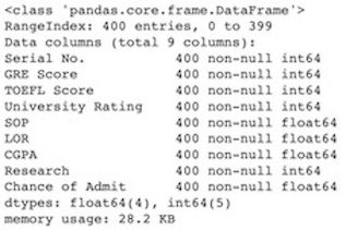
Looking at the data using the Pandas.dataframe .head() and .info() methods we obtain the following outputs.


The dataset contains information about 400 observations related to 9 features (GRE Scores, TOEFL Scores, University Rating, Statement of Purpose Strength, Letter of Recommendation Strength, Undergraduate GPA, Research Experience, Chance of Admit) which are all numeric. There is no missing values.
By using the .describe() method we can get some summary statistics to get an idea of the distribution of the features in the dataset.

The distribution of the features in the sample seems have no issue.
We can move to the next step: extracting features (X) and label (y, i.e. the variable to predict) and split the whole dataset in a training and a test set.
y = adm['Chance of Admit ']
X = adm.iloc[:,1:8]
X_train, X_test, y_train, y_test = train_test_split(X, y, test_size = 0.2, random_state = 123)
The following code instantiate an object of the class RandomForestRegressor with default setting parameters.
randomForest = RandomForestRegressor(random_state =123 )
Then, the model is trained using the training sample.
randomForest.fit(X_train, y_train)
Once the model built, it is used to predict the target variable using the test sample.
y_pred = randomForest.predict(X_test)
To assess the model performance, different metrics can be used:
• Mean absolute error (MAE)
• Mean squared error (MSE)
• R-squared scores
• Adjusted R-squared scores (which is not a built-in metric and we have to compute it manually)
mae = mean_absolute_error(y_test, y_pred)
mse = mean_squared_error(y_test, y_pred)
r2 = r2_score(y_test, y_pred)
adj_r2 = 1 - (1 - r2)*(X_train.shape[0] - 1)/(X_train.shape[0] - X_train.shape[1] - 1)
# Print metrics
print('Mean Absolute Error:', round(mae, 2))
print('Mean Squared Error:', round(mse, 2))
print('R-squared scores:', round(r2, 3))
print('Adj.R-squared scores:', round(adj_r2, 3))

The next step is to explore how tuning model’s hyperparameters can affect its performance in making prediction. We consider the Adjusted R-squared score as metric to evaluate the model.
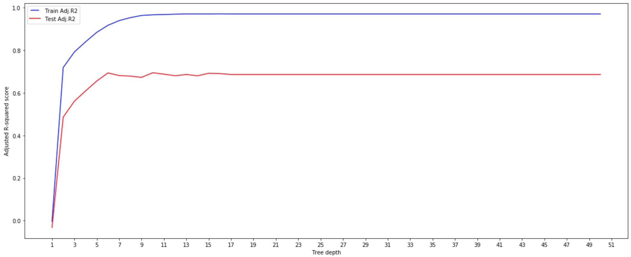
- max_depth

We can see that above a certain depth the model starts overfitting. It perfectly predicts all the train data (the Adjusted R2 for the training set is 1) but its predictions are not accurate over the test set.
With a max_depth of 10, the model gets the highest Adjusted R2 (0.695).
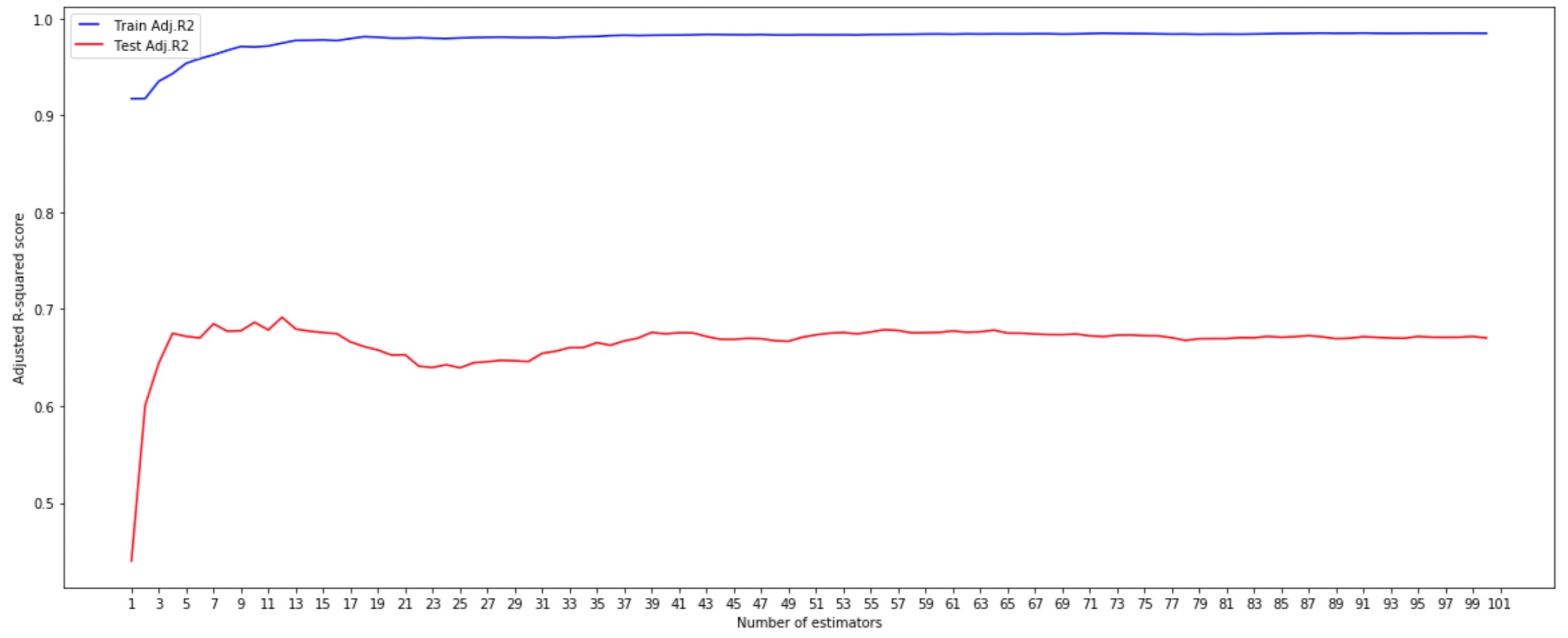
- n_estimators

We can see that adding a high number of trees doesn’t necessarily improve model accuracy. In this case, with 12 estimators, our model gets the highest Adjusted R2 (0.692).
- max_features

We have implemented the model by tuning only the max_features parameter with different settings, namely ‘None’, ‘sqrt’, ‘log2’ , ‘int’ (3) and ‘float’ (0.5).
We can see that, in this case, even if with slight differences, setting the parameter using a customized integer number or a customized fraction of features allow to get a highest Adjusted R-squared.
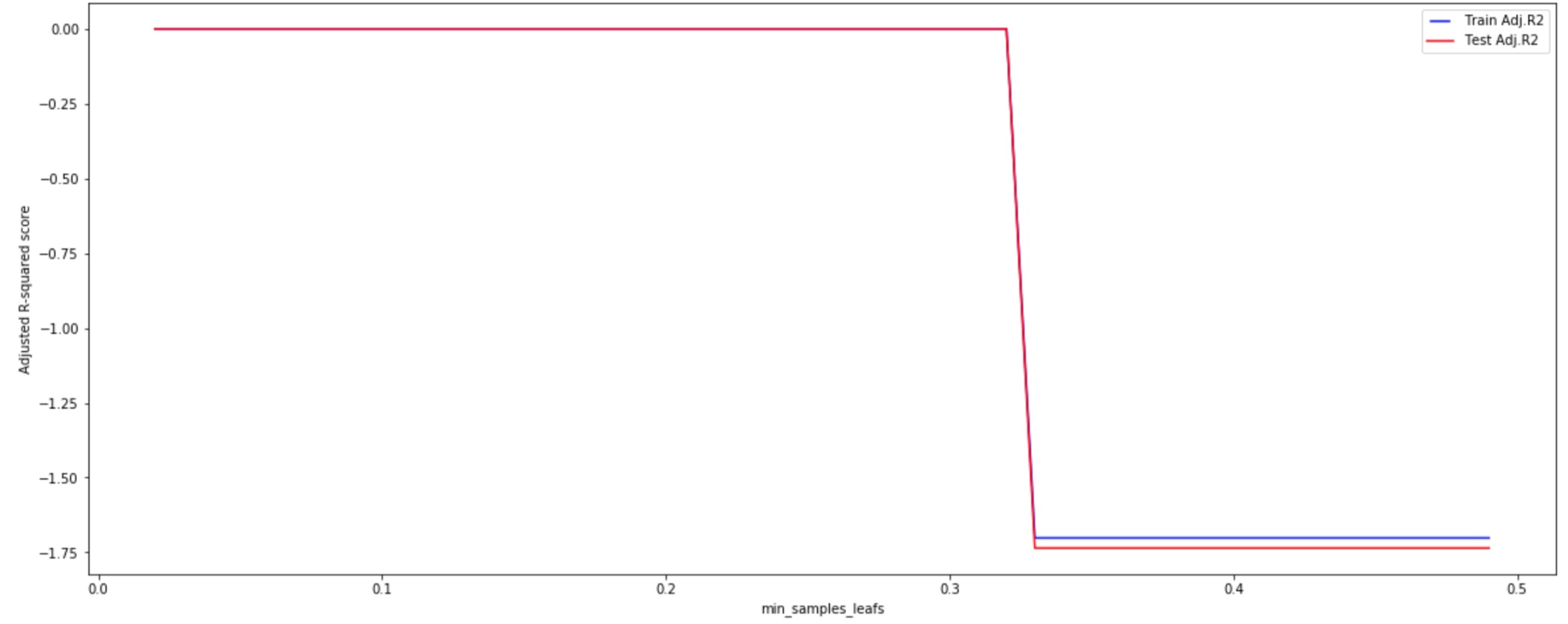
- min_samples_leaf

Increasing the number of data points allowed in the end node leads the model to make not accurate predictions, both on the training and the test set.
In this case with a minimum of 20% of our test data in each leaf node, the model gets an Adjusted R-squared score equals to 0.68.
We can now modify our previous model by tuning its parameters according to our findings.
randomForestTuned = RandomForestRegressor(max_depth = 10, max_features=0.5, n_estimators=12,\
              min_samples_leaf=0.02, random_state=123)

When looking at the model evaluation’s metrics we can see that its performance is improved and the Adjusted R-squared is increased from 0.661 to 0.721.
To end this article, I would like to suggest a very interesting paper about Random Forest hyperparameters “Hyperparameters and Tuning Strategies for Random Forest” by Philipp Probst, Marvin Wright and Anne-Laure Boulesteix. Even if it is focused on implementation of tuning using R rather than Python, it is a useful source for further study.
