Data Pre Processing for Machine Learning with Python

This article is the first of a series dedicated to the machine learning workflow using a dataset retrieved from a Kaggle competition entitled House Prices: Advanced Regression Techniques and available here.
The dataset contains information from the Ames Assessor’s Office on residential property sales that occurred in Ames, Iowa from 2006 to 2010.

The aim is to build a model to predict the price of a home based on 81 explanatory variables describing (almost) every aspect of residential homes in Ames, Iowa.

The code is written in Python and it is available here.

The Machine Learning Worflow

Any machine learning project should follow those steps (often in an iterative way):

• Step 1 – State the question and determine required data
  
• Step 2 – Acquire the data in an accessible format
  
• Step 3 – Loading the required libraries and modules
  
• Step 4 – Loading the data
  
• Step 5 – Exploratory Data Analysis (EDA)
  
• Step 6 – Data Cleaning and Data Pre-Processing
  
• Step 7 – Split data into training and test set
  
• Step 8 – Build and training the model
  
• Step 9 – Test the model: making Predictions
  
• Step 10 – Evaluate the model
  

In this part we will focus on the tasks required to prepare the data for analysis and any further operation (i.e. we will cover steps from 1 to 7).

Since the research question has been already stated in the introduction, let’s start from the second step.

Loading the required libraries and modules

import pandas as pd 
import numpy as np
import matplotlib.pyplot as plt
import seaborn as sns

The Numpy package is for performing Mathematical operations, the Pandas package is for manipulating dataset, pyplot and seaborn for data visualization. Throughout the project we’ll use different packages from sklearn (a Python library dedicated to machine learning).

Loading the data

From the source, data have already been split into train and test set. Therefore, at this stage, we load only the train set.

df = pd.read_csv("train.csv")
df.sample(3)

The dataframe .shape attribute allows to view the number of samples and features we’re dealing with.

df.shape

Our dataset contains 1460 observation and 81 explanatory variables.

Exploratory Data Analysis

Exploratory data analysis is a crucial step in any data workflow. The key purpose of EDA is to examine the dataset in order to:
• map out the underlying structure of that data and identify potential patterns
•   generate hypotheses for further analysis
•   identify missing values
•   highlight outliers

Different techniques can be used to perform Exploratory Data Analysis:

• Univariate analysis and visualization, which provides summary statistics for each feature in the dataset
  
• Bivariate analysis and visualization, which allows to explore the relationship between each variable in the dataset and the target variable of interest
  
• Multivariate analysis and visualization, which allows to understand interactions between different features in the dataset
  
• Dimensionality reduction, which helps to understand which features account for the most variance between observations and to feature selection
  

Becoming familiar with the features

It’s important to understand what feature each column represents, in order to avoid to make mistakes in the data analysis and the modeling process.

The dataset comes with a data dictionary containing a description of each feature along with the list of allowed values.

We can create a function to display its contents as follows

def read_description(file_name):
    f = open(file_name, "r")
    
    lines = f.readlines()

    for i in lines:
        print(i)

We can also take advantage of the pandas .info() method which displays for each column:

•   its name
•   the number of non-null observation
•   the data type.

An overview of the output is displayed below

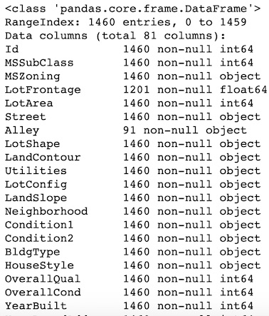
As we can see from the output, the dataset contains a miscellany of float, integer and object data types as well as several columns having missing values (we’ll come back to this issue later).

In order to understand which feature each column actually represents (and if the current data type is suitable to describe it) we have to refer to the data dictionary by calling the function read_description() created above.

read_description("data_description.txt")

The output looks like this

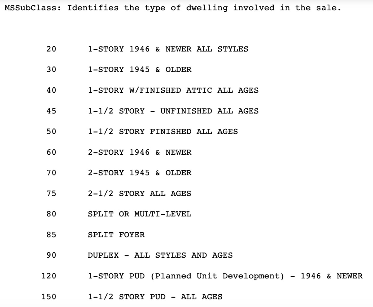
Based on this information, we can split up the features into 4 different sets according to their nature.

• Continuous features (such as SalePrice, LotFrontage, GarageArea, etc)
  
• Discrete features (such as BsmtFullBath, BsmtFullBathAbvGrd, Fireplaces, etc)
  
• Nominal Categorical features (such as MSSubClass, Neighborhood, Heating, etc)
  
• Ordinal Categorical features (such as OverallQual, HeatingQC, YearBuilt)
  

We consider nominal and ordinal features separately for make easier the encoding step at the pre-processing stage.

The MSSubClass variable, which identifies the type of dwelling involved in the sale, is coded as an integer but it is actually a categorical variable. For that, we recode its as a cateogorical variable.

df['MSSubClass'] = df['MSSubClass'].astype('category')

We remove the ‘Id’ column and reorganize the other according to the following order:

• first continuous and discrete features
  
• then categorical and ordinal features
  

For that, we start creating a list of features for each type of variable. Then, we concatenate these lists in one single list called new_columns_order and finally we pass this list as argument to the dataframe .reindex() method.

continuous_features = ['SalePrice','LotFrontage', 'LotArea',\
'MasVnrArea', 'BsmtFinSF1', 'BsmtFinSF2','BsmtUnfSF',\ 
'TotalBsmtSF', '1stFlrSF', '2ndFlrSF', 'LowQualFinSF',\
'GrLivArea', 'GarageArea', 'WoodDeckSF', 'OpenPorchSF',\
'EnclosedPorch','3SsnPorch', 'ScreenPorch','PoolArea',\
'MiscVal']
discrete_features = ['BsmtFullBath', 'BsmtHalfBath',\
'FullBath', 'HalfBath', 'BedroomAbvGr','KitchenAbvGr',\
'TotRmsAbvGrd','Fireplaces', 'GarageCars']
nominal_features = ['MSSubClass', 'MSZoning', 'Street',\
'Alley','LotShape', 'LandContour', 'Utilities','LotConfig',\
'LandSlope', 'Neighborhood','Condition1', 'Condition2',\
'BldgType','HouseStyle','RoofStyle', 'RoofMatl','Exterior1st',\
'Exterior2nd', 'MasVnrType','Foundation', 'Heating', 'CentralAir',\
'Electrical', 'SaleType','SaleCondition','Functional', 'GarageType',\
'GarageFinish', 'PavedDrive','MiscFeature']
ordinal_features = ['OverallQual','OverallCond','ExterQual','ExterCond',\
'BsmtQual', 'BsmtCond','BsmtExposure', 'BsmtFinType1', 'BsmtFinType2',\ 
'HeatingQC','KitchenQual', 'FireplacesQu', 'GarageQual', 'GarageCond',\
'PoolQC', 'Fence', 'YearBuilt', 'YearRemodAdd', 'GarageYrBlt', 'MoSold',\
'YrSold' ]

new_columns_order = continuous_features + discrete_features +\
					nominal_features +  ordinal_features

df = df.reindex(columns=new_columns_order)

Univariate Exploratory Analysis on numeric features

After understanding what kind of information are available, we have to get an idea of how these features are distributed inside our dataset.

We start from the continuous features which relate measurements of area dimensions for each observation. For each of them we compute some summary statistics and we plot their distribution.

df[continuous_features].describe()

df[continuous_features].hist(figsize = (30,30), bins = 15);

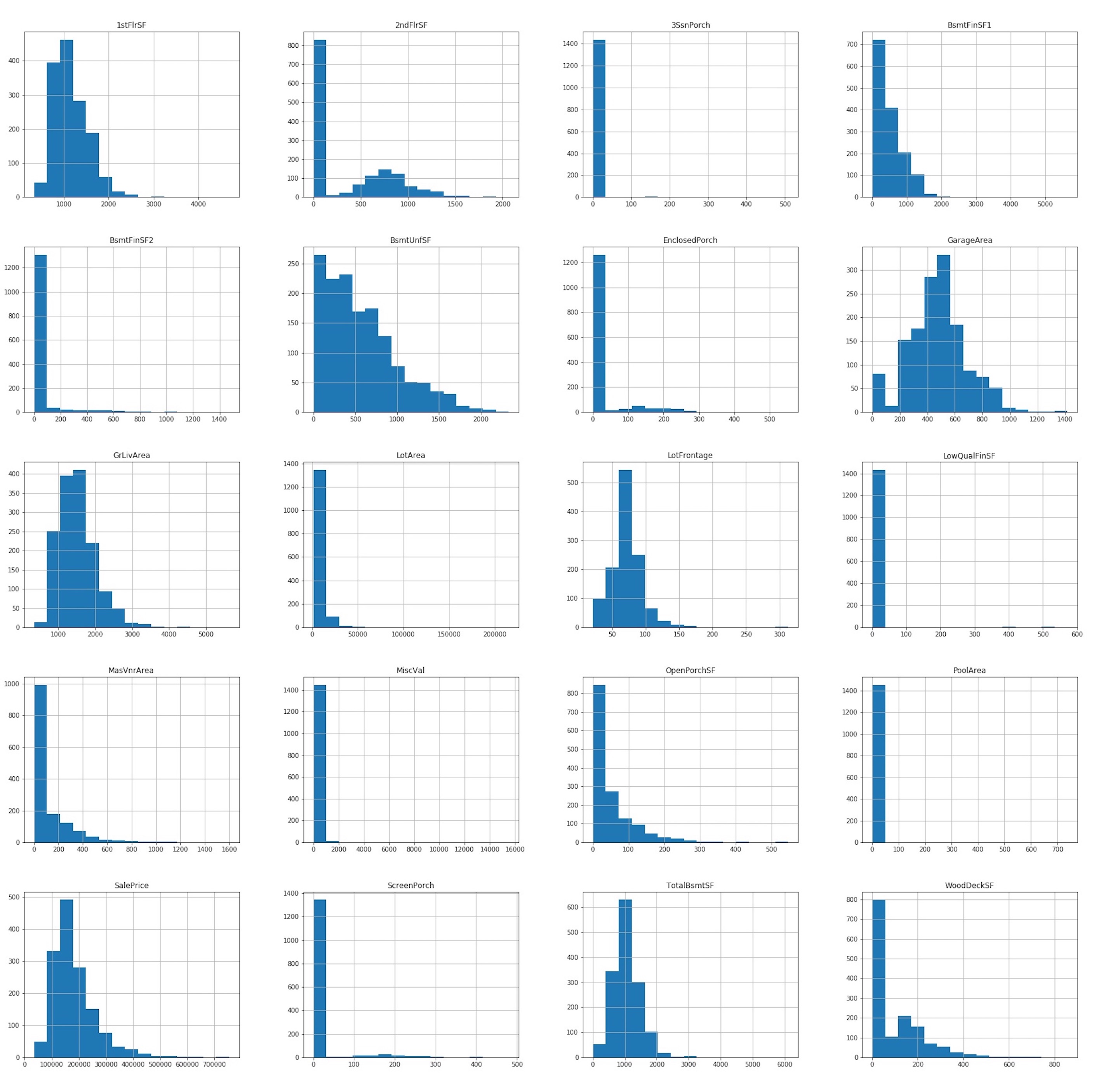
Any of our continuous features follows a normal distribution, except for the TotalBsmtSF variable which is quite close to a gaussian.
Some of them are right skewed like 1stFlrSF, 2ndFlrSF. Also the 2ndFlrSF feature for most of the observation takes value zero, meaning that many properties in our sample have no a second floor.

Others have most of the observations concentrated at the lower end of the distributions and few at the other end, resulting in a distribution with a lot of empty space (like 3SsnPorch, ScreenPorch or PoolArea). This may be due to the existence of outliers.

The first impression about our sample is that most of the properties sold are one-floor houses, with a prevalence of open porch and wood deck solutions to extend outdoor living areas, and a prevalence of unfinished over finished basements area. Also, 50% of properties has a living area above ground between 1130 and 1777 square feets and a garage area between 335 and 576 square feets. Very few of them have additional features such as pool or other facilities like elevator, a second garage etc.

Let’s take a closer look to our target variable ‘SalePrice’

plt.hist(df['SalePrice'], bins = 40);

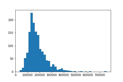
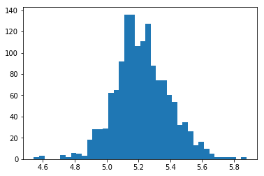
It’s clear that SalePrice doesn’t follow normal distribution, so before performing regression it has to be transformed.

df['SalePrice'] = np.log10(df['SalePrice'])

The resulting distribution is displayed below

Next, we consider discrete features.

df[discrete_features].describe()
df[discrete_features].hist(figsize = (30,30), bins = 30);

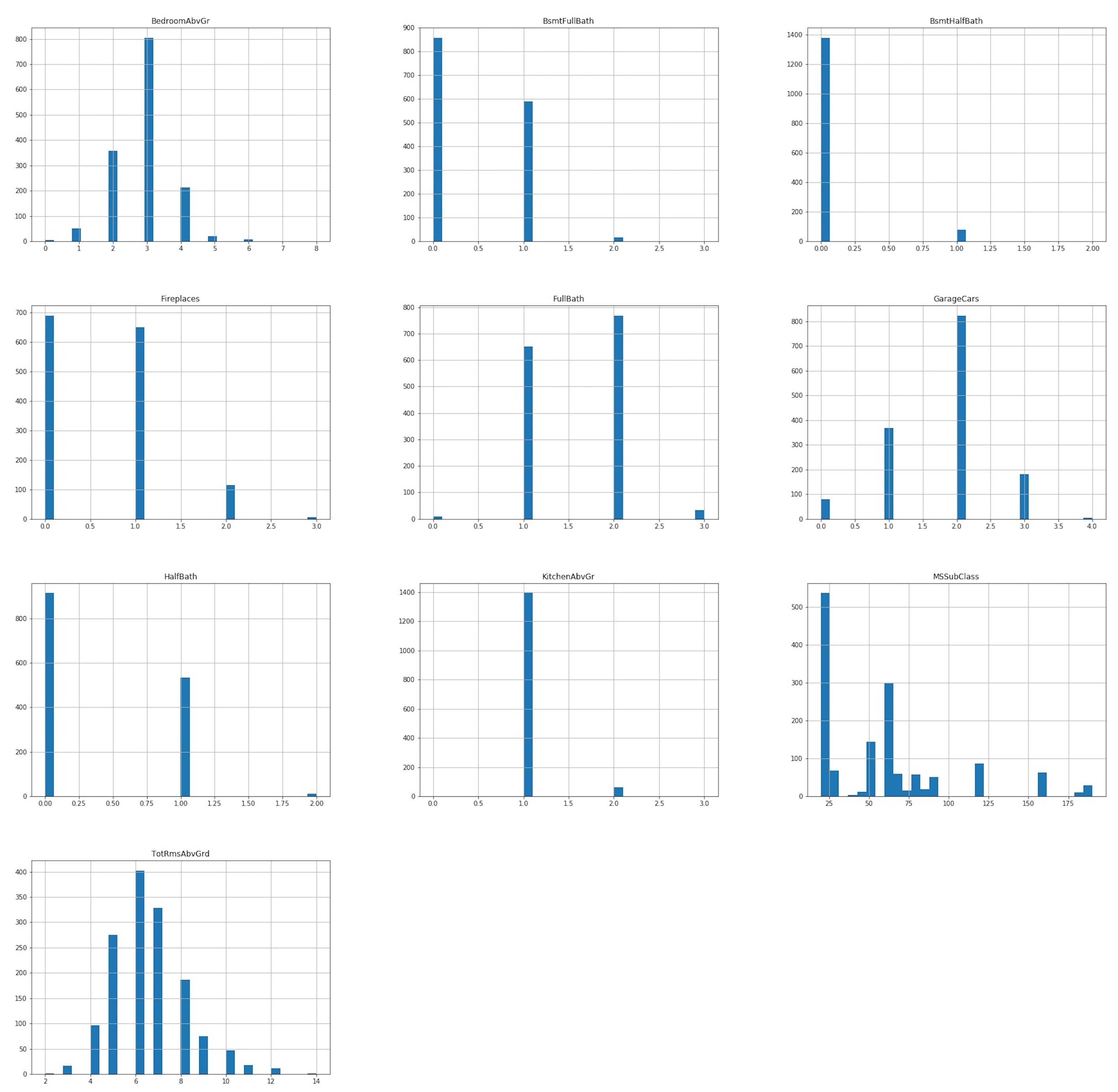
The discrete variables mostly have to do with the number and kind of rooms, as well as the number of fireplaces or the size the garage, in cars capacity, that a given property has.

The majority of the properties sold have between 5 and 7 rooms above the ground, with 2 or 3 bedrooms and 1 or 2 full bathrooms (and any half or full basement baths). The median size of garages is of 2 cars capacity and more than 50% of the properties has a fireplace.

Univariate Exploratory Analysis on categorical features

We define a function bar_plot() to plot multiple barplot at once. Then, we just need to call this function and pass the different subset of our feature we want to visualize.

def bar_plot (df, features, rows, cols, hfig, wfig):
    fig = plt.figure(figsize = (hfig,wfig))
    for i, feature_name in enumerate(features):
        ax = fig.add_subplot(rows, cols, i +1)
        sns.countplot(x = feature_name, data = df)
        plt.xticks(rotation = 90);
    fig.tight_layout()

Starting from Nominal variables, we can split them up into different groups, based on property’s features they represent:

•   A first group relate property location. Variables belonging to this group are ‘MSZoning’, which identifies the general zoning classification of the sale (such as commercial, residential, etc), ‘Neighborhood’ (i.e. the physical location of a property within Ames city limits), ‘Condition1’ and ‘Condition2’ (which describes if the property is located near to various conditions such as arterial street, railroad, park, etc.).

We store those variables in a list and we pass that list to the bar_plot function.

location = ['MSZoning','Condition1', 'Condition2', 'Neighborhood']
bar_plot (df, location, int(len(location)/2)+1, 2, 12, 10)

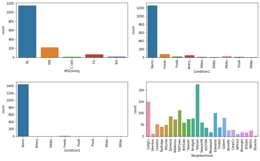
Considering this first group, we see that 94% of the properties in our sample are located in a residential (medium and lower density) zone and 86% of properties have a normal proximity to various city conditions. The ‘Neighborhood’ variable will be explored later with reference to the SalePrice.

•   The second group of the nominal variables identifies:

• structural characteristics of the property, including lot configuration, general shape and flatness of the property, type of access to the property (street, alley and whether they are paved), the garage location as well as if its interior is finished.
  
• structural characteristics of the dwelling, such as the type of building, the house style, the type of foundation, which is the exterior siding, which is the type of the roof and the material is made of, the masonry veneer type (if any).
  
• property’s utilities, such as which kind of public utilities are available, the type of heating and electrical system, if there is central air conditioning and other miscellaneous features.
  

We store those variables in 3 different lists and we pass each of them to the bar_plot function.

strucCaractProp = ['LotShape','LandContour', 'LandSlope', 'LotConfig',\
                         'Street', 'Alley', 'PavedDrive', 'GarageType', 'GarageFinish']


strucCaractDwel = ['MSSubClass','BldgType','HouseStyle','Foundation','RoofStyle','RoofMatl',\
                         'MasVnrType', 'Exterior1st', 'Exterior2nd']

utilities = ['Utilities','Heating', 'CentralAir', 'Electrical', 'MiscFeature','Functional']

bar_plot (df, strucCaractProp, int(len(strucCaractProp)/2)+1, 2, 12, 18)

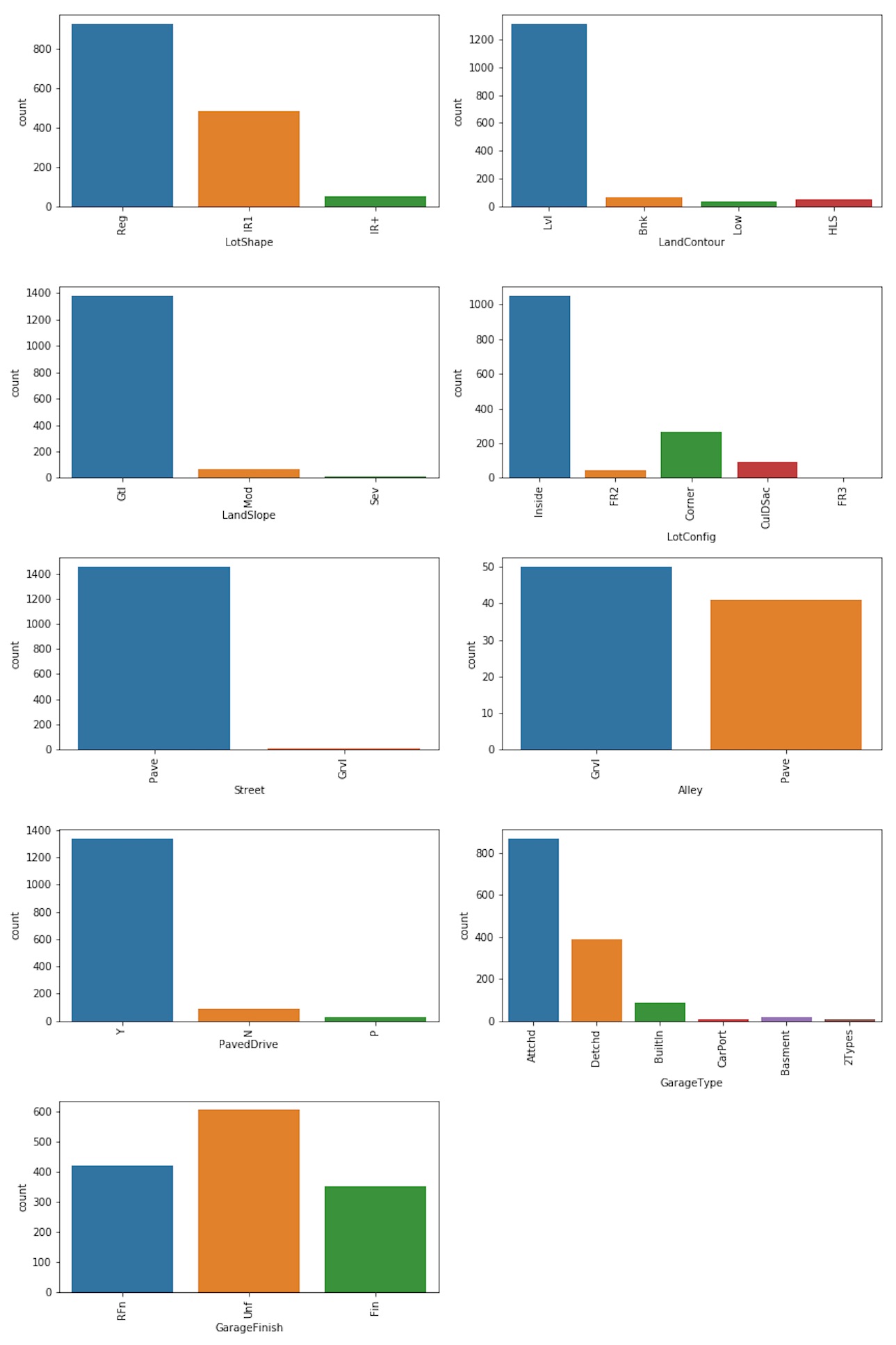
Looking at the lot shape we can see that 64% of properties were a regular shape whereas 33% were slightly irregular. We may consider to regroup the other two categories of the variable lot of shape into a new category “IR+”.

df.loc[(df.LotShape == 'IR2'),'LotShape'] ='IR+'
df.loc[(df.LotShape == 'IR3'),'LotShape'] ='IR+'

Also, most of the properties are located on a flat land and the most common type of lot configuration is the interior lot (i.e. a property which lies between homes on the left and right side, facing the street on only the frontal side). When considering the variables related to the garage we can see that the majority of the properties has an attached garage with an unfinished interior.

bar_plot (df, strucCaractDwel, int(len(strucCaractDwel)/2)+1, 2, 12, 20);

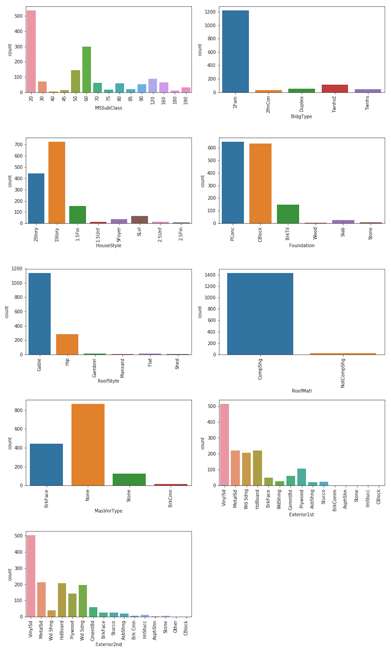
The HouseStyle and MSSubClass variables provide pretty much the same information: most of the properties sold were one or two-level single-family detached dwelling.

Most of the properties had foundation made of poured Contrete or cinder Block.

Since 98% of roof material is Standard (Composite) Shingle we may regroup the other seven categories to into a NotCompShg category.

df.loc[df['RoofMatl'] != 'CompShg', 'RoofMatl'] = 'NotCompShg'

bar_plot (df, utilities, int(len(utilities)/2)+1, 2, 9, 10);

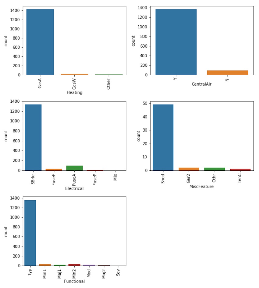
Since 99% of the observations in our sample have all public utilities available, the feature ‘Utilities’ is not informative and we can drop it.

df.drop('Utilities', axis = 1, inplace = True)

Since 98% of heating types are either GasA (Gas forced warm air furnace) or GasW (Gas hot water or steam heat) we keep those categories and group the other into an ‘other’ class.

other = {'Grav': 'Other', 'Wall': 'Other', 'OthW': 'Other', 'Floor': 'Other'}
df['Heating'].replace(other, inplace = True)

•   The third group relate sale characteristics, such as the type of sale and the sale conditions

sale = ['SaleType','SaleCondition']

bar_plot (df,sale,2, 2, 12, 7)

In our sample, 87% of properties were purchased from a former owner through a warranty deed whereas 8% were new homes just constructed and sold.

We regroup the other categories into a single category.

otherType = {'COD': 'Other', 'ConLD': 'Other', 'ConLw': 'Other', 'ConLI': 'Other', 'CWD': 'Other',\
             'Oth': 'Other', 'Con': 'Other'}
df['SaleType'].replace(otherType, inplace = True)

When considering the condition of sale, we see that 82% of properties were sold through a normal sale, it was a partial sale for 9% of the properties (this is may be related to the new homes) and 7% are sold under abnormal sale conditions (e.g. foreclosure).

After checking the median sale price across the different categories as follows

df.groupby('SaleCondition')['SalePrice'].median()

we regroup the remaining categories into a the ‘normal’ category.

otherCond = {'AdjLand':'Normal', 'Alloca':'Normal', 'Family':'Normal'}
df['SaleCondition'].replace(otherCond, inplace = True)

Ordinal variables

Ordinal variables are ratings of the quality and condition of the properties as a whole and of single rooms or utilities. In this category were also considered the year in which the property was built or remodelled and the month and year when the sale was made.

We start by examining the month of sale, to figure out if there is a seasonality in sales.

sns.countplot(df['MoSold']);

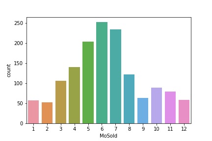
65.35% of the properties were sold between april and august.

A useful information can be provide by the age of the house at the time it was sold, that can be calculated as follows

df['HouseAge'] = df['YrSold'] - df['YearBuilt']

plt.figure(figsize = (20,5))
sns.countplot(df['HouseAge'])
plt.xticks(rotation = 90);

Most of the properties were sold one year after building.

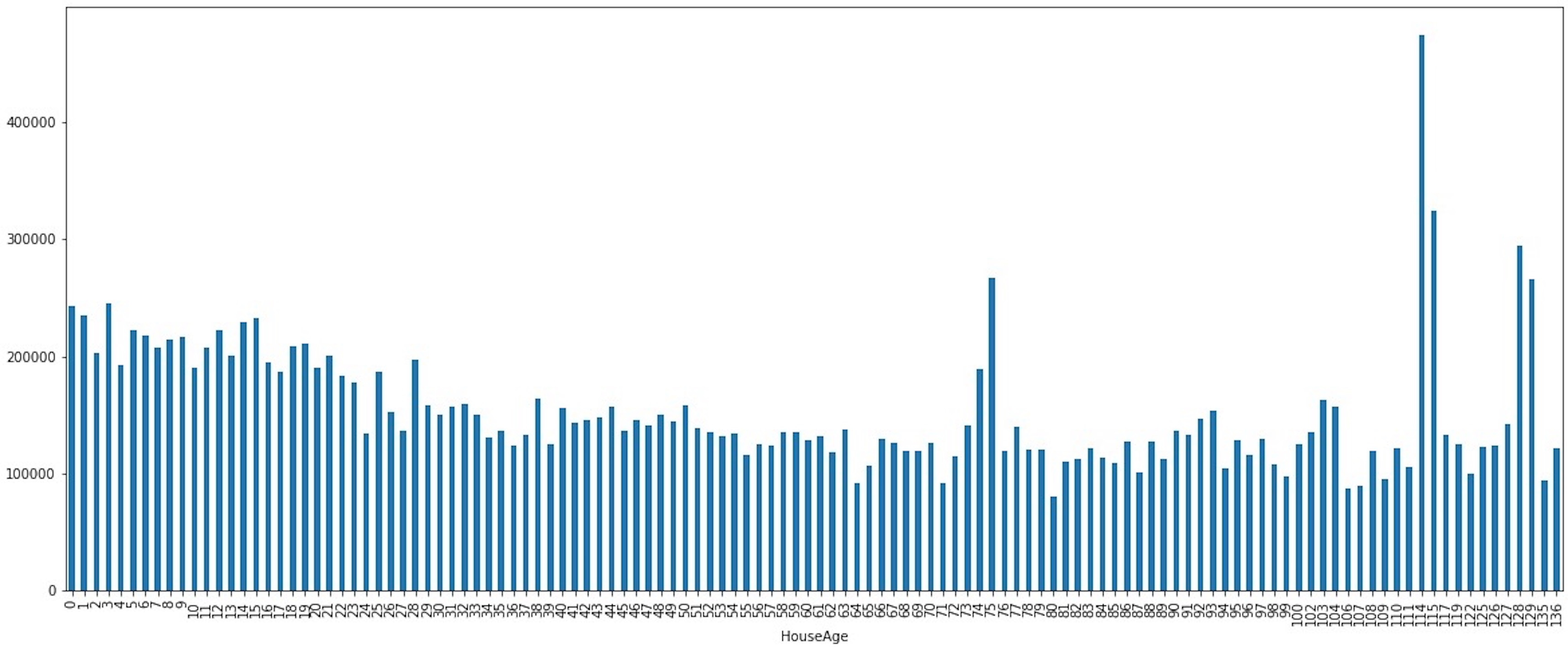
We can also visualize the variability of the median price of sale based on the house age.

df.groupby("HouseAge")['SalePrice'].median().plot(kind = 'bar', figsize = (20,8))

Bivariate Exploratory Analysis on numeric features

The next step is to understand which features are the most correlated with the target variable (in order to find out which feature can be use as predictors in our model) and which are correlated each other (in order to prevent multicollinearity).

For that we build a function to visualize how numeric features are correlated to the target variable through a scatter plot. We use the .regplot() method in seaborn.

def scatters (df, features, rows, cols):
    fig = plt.figure(figsize = (10,30))
    for i, feature_name in enumerate(features):
        ax = fig.add_subplot(rows, cols, i +1)
        sns.regplot(x = feature_name, y= 'SalePrice', data = df);
    fig.tight_layout()

We analyse continuous and discrete numeric features separately.

scatters(df, continuous_features[1:], int(len(continuous_features[1:])/2)+1,2)

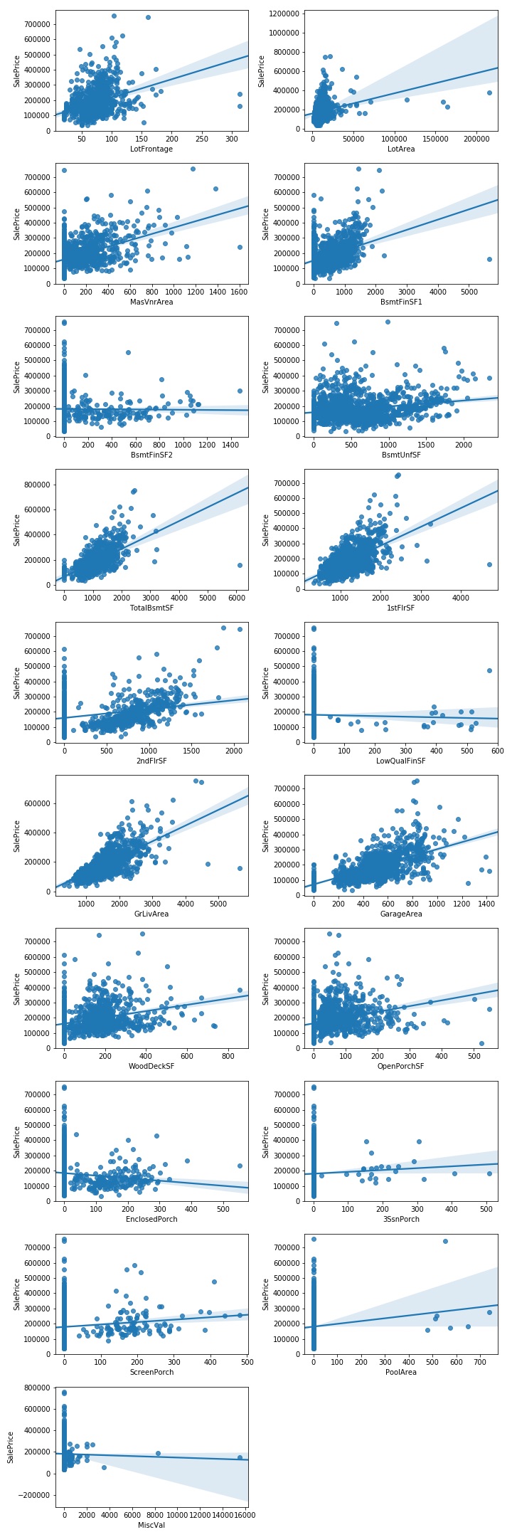
From the plots above, it seems that the target variable is linearly correlated with the GrLivArea, 1stFlrSF and GarageArea features. However, they don’t provide information about the strenght of these correlations.

For that we can plot an heatmap, available in the seaborn package.

corr_continuous = round(df[continuous_features].corr(),2)
plt.figure(figsize= (15, 15))
mask = np.zeros_like(corr_continuous, dtype=np.bool)
mask[np.triu_indices_from(mask)] = True;
sns.heatmap(corr_continuous, mask=mask, annot = True, linewidths=.5);

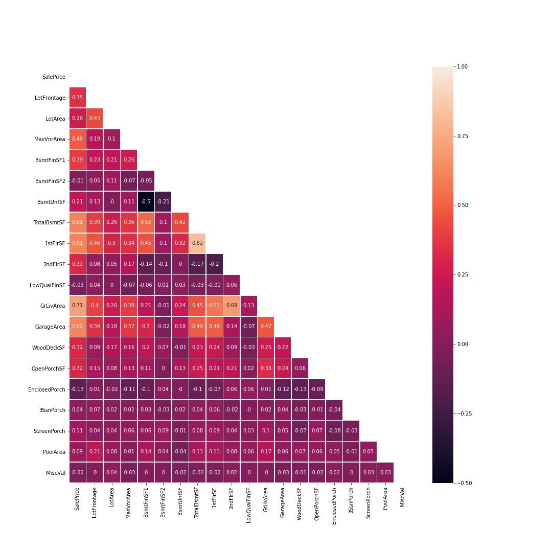
The correlation matrix confirms the scatterplots’ results: the continuous variables most correlated to our target variable (in order of strenght of correlation) are GrLivArea, GarageArea, 1stFlrSF, TotalBsmtSF.
However, GrLivArea and 1stFlrSF are also correlated each other, like 1stFlrSF and TotalBsmtSF.

scatters(df, discrete_features, int(len(discrete_features)/2)+1,2);

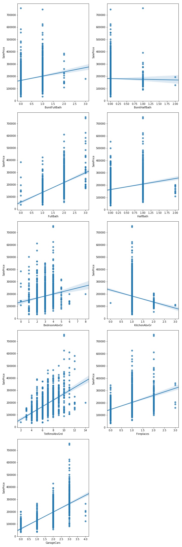
From the plot above, it seems that the target variable is linearly correlated withFullBath, TotRmsAbcGrd, Fireplaces and GarageCars featues.

corr_discrete = round(df[['BsmtFullBath','BsmtHalfBath','FullBath','HalfBath','BedroomAbvGr',\
                          'KitchenAbvGr','TotRmsAbvGrd','Fireplaces','GarageCars','SalePrice']].corr(),2)
plt.figure(figsize= (8, 8))
mask = np.zeros_like(corr_discrete, dtype=np.bool)
mask[np.triu_indices_from(mask)] = True;
sns.heatmap(corr_discrete, mask=mask, annot = True, linewidths=.5);

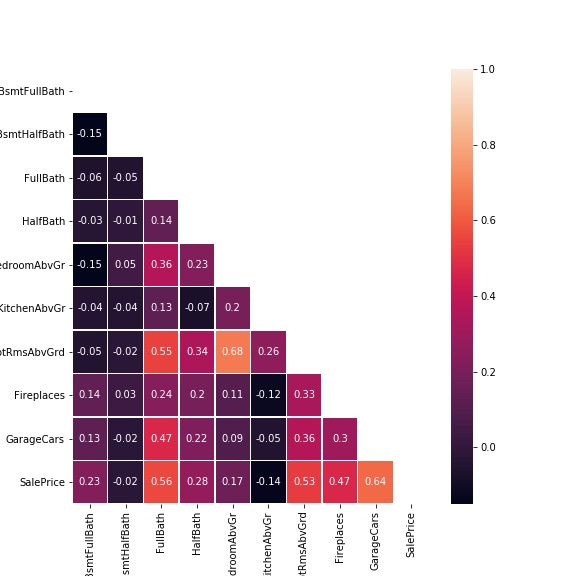
The correlation matrix confirms the initial thoughts. However, FullBath and TotRmsAbcGrd are also correlated each other.
The variable with the stronger correlation is GarageCars (for the other the correlation is weaker).

Visualizing relationships between categorical features and target variable

The same way, we build a function to visualize the relationship between categorical features and to the target variable through boxplots as follows

def boxplots (df, features, rows, cols):
    fig = plt.figure(figsize = (15,70))
    for i, feature_name in enumerate(features):
        ax = fig.add_subplot(rows, cols, i +1)
        sns.boxplot(x = feature_name, y= 'SalePrice', data = df)
        plt.xticks(rotation = 90);
    fig.tight_layout()

We start plotting the target variable’s distribution across nominal features

boxplots(df, nominal_features, int(len(nominal_features)/2)+1 ,2)

Moving to ordinal features

ordinal_features = ['OverallQual','OverallCond','ExterQual', 'ExterCond', 'BsmtQual', 'BsmtCond',\
 'BsmtExposure', 'BsmtFinType1', 'BsmtFinType2', 'HeatingQC', 'KitchenQual', 'GarageQual', 'GarageCond',\
 'Fence', 'YearBuilt', 'YearRemodAdd', 'MoSold', 'YrSold']

boxplots(df, ordinal_features, int(len(ordinal_features)/2)+1 ,2)

The categorical features for which the SalePrice shows the highest variability are:

• OverallQuality
  
• MSZoning
  Properties sold in Floating Village Residential (FV) zone have the highest median SalePrice compared to other zones. However, for properties sold in the Residential Low Density (RL) zone the SalePrice distribution is right skewed with many observations having high SalePrice.

• Neighborhood
  When considering Neighborhood, we see that the median SalePrice is highly variable depending on the neighbourhood. Also, Northridge and Northridge Heights are those with the highest median SalePrice followed by the Stone Brook neighbourhood.

• Condition1 and Condition2
  Proximity to off-site feature like park, greenbelt, etc. as well as to railroad leads to a higher median SalePrice.

• BldgType
  When considering the type of building, the Single-family Detached and the Townhouse End Unit dwelling are those with the highest median SalePrice.

• HouseStyle
  Two-level properties as well as split-level house have the highest median SalePrice

• HouseAge
  It is one of the features determining the highest variability in the SalePrice

• Exterior1st and ExternalQual
  Among the different materials for external siding, Imitation stucco, stone and cement board are those which are related to the highest median SalePrice. This may be due to the fact that they ensure high durability.

• GarageType
  Built-In garages (which are part of the house) have the highest median SalePrice. This may be due to the fact that they typically have a room above them, allowing to increase the total living area of a property.

• GarageFinish
  
• Heating and HeatingQC
  Based on type of heating, the GasA type has the highest median SalePrice. Also the quality of the heating system has a high impact on SalePrice

• CentralAir
  Also, the presence of central air conditioning seems to be an important feature in determing SalePrice level.

• Electrical
  When considering the Electrical system, Standard Circuit Breakers & Romex is what ensure the highest SalePrice

• MiscFeature
  Among the Miscellaneous Features, the availability of a tennis court seems to have the highest impact on the median selling price, followed by the availability of a second garage.

• SaleType
  New home are sold at a highest price than others.

• SaleCond
  Properties sold under partial condition (Home not completed yet) have the highest median SalePrice (it is related to the fact that are new properties).

Data Cleaning and Pre-Processing.

It’s now time to preparing the data for analysis. It mainly means

•   Deal with missing data
•   Deal with outliers
•   Deal with categorical data
•   Scaling the features

Dealing with missing data

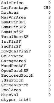
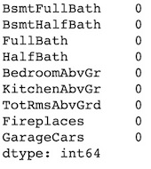
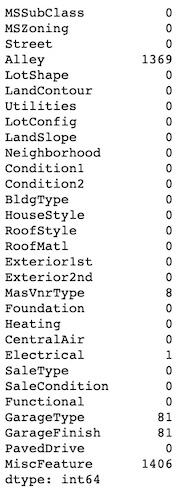
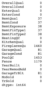
We can check how many missing value a column has by concatenatig the .isnull() and the .sum() methods. We perform this operation on the 4 subsets of features by using indexing selection on the dataframe.

df[continuous_features].isnull().sum()

df[discrete_features].isnull().sum()

df[nominal_features].isnull().sum()

df[ordinal_features].isnull().sum()

Let’s examine one feature having missing values at a time.

• We know, from the data dictionary that GarageType, Fence, MiscFeature and Alley variables have ‘nan’ values when the property lacks those features.

We can create an additional category “No feature” and encoding those missing values to the new category.

df['GarageType'].fillna("No Garage", inplace = True)
df['Fence'].fillna("No Fence", inplace = True)
df['MiscFeature'].fillna("No MiscFeature", inplace = True)
df['Alley'].fillna("No Alley", inplace = True)

Missing values for other categorical/ordinal variables related to GarageType such as GarageQual, GarageCond and GarageFinish can be handled in the same way.

However, for the GarageYrBlt variable, this approach is not suitable and since no valid value can be inputated (since it is not logical to have a year of built for something never been built) we may consider to drop those feature.

df.drop('GarageYrBlt', axis=1, inplace = True)

• As for the previous variables, BsmtQual, BsmtCond, BsmtExposure, BsmtFinType1, BsmtFinType2 have missing values when a property has no basement. Therefore, we can use the same encoding and create an additional category “None”.

However, one observation (id 948) has a missing value for the BsmtExposure variable and another one (id 332) has a missing value for the BsmtFinType2 variable even if the value of the TotalBsmtSF variable (Total square feet of basement area) for those observations is different from zero (meaning that they actually have a basement).

We can check which values other basement related variables take for those observations and which is the most common value for the variables having missing values for other observations having the same values of related variables.

Starting with the observation having Id 948

df[df.index == 948][["BsmtExposure","BsmtCond","BsmtFinSF1",\
"BsmtFinType1","BsmtFinSF2", "BsmtFinType2", "BsmtUnfSF",\
"TotalBsmtSF"]]

df[(df["BsmtCond"] == 'TA')& (df['BsmtFinType1'] == "Unf")&\
	(df["BsmtFinType2"] == 'Unf')]\
	['BsmtExposure'].value_counts()

We can assume that the Id 948 has an ‘Normal’ basement exposure and impute this value.

df.at[948, "BsmtExposure"] = "No"

Moving to the observation having Id 332

df[df.index == 332][["BsmtExposure","BsmtCond",\
					"BsmtFinSF1","BsmtFinType1",\
                     "BsmtFinSF2", "BsmtFinType2",\
                     "BsmtUnfSF", "TotalBsmtSF"]]

df[(df["BsmtExposure"] == 'No')&(df["BsmtCond"] == 'TA')\
	& (df['BsmtFinType1'] == "GLQ")]['BsmtFinType2'].value_counts()

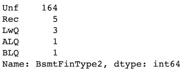
We can assume that the Id 332 has an Unfinished basement and impute this value.

df.at[332, "BsmtFinType2"] = "Unf"

Finally, we encoding the missing values for the other basement variables to the “None” category.

df["BsmtQual"].fillna("None",inplace = True)
df["BsmtCond"].fillna("None",inplace = True)
df["BsmtExposure"].fillna("None",inplace = True)
df["BsmtFinType1"].fillna("None",inplace = True)
df["BsmtFinType2"].fillna("None",inplace = True)

• For the variable Electrical, which has only one missing value, we can impute a value using deduction. We can check the year this property has been built and which kind of electrical systems the other properties built the same year have.

df[df['Electrical'].isna()]['YearBuilt']

df[df['YearBuilt'] == 2006]['Electrical'].value_counts()

Since all those properties have a Standard Circuit Breakers & Romex, we can assume that our record missing this value has the same kind of electrical circuit.

df['Electrical'].fillna("SBrkr", inplace = True)

• For MasVnrType column we impute “No MasVnr” and for the related MasVnrArea we impute 0.0

df['MasVnrType'].fillna("No MasVnr", inplace = True)

df['MasVnrArea'].fillna(0.0, inplace = True)

• For the LotFrontage variable, we can impute missing values using the pandas .interpolate() method. Interpolation is a mathematical method that adjusts a function to the data and uses this function to extrapolate the missing data.
In this case a good approximation may be a linear method.

df['LotFrontage'].interpolate(method='linear', inplace = True)

• For FireplacesQu and PoolQC columns, since almost all values are missing we can drop the whole column.

df.drop(["FireplacesQu", "PoolQC"], axis = 1, inplace = True)

After these operations, the former list of ordinal features in our dataset has changed (we have removed GarageYrBlt, FireplacesQu and PoolQC variables) and we need to update it since we will use it again in the next step.

ordinal_features = ['OverallQual','OverallCond','ExterQual',\
'ExterCond', 'BsmtQual','BsmtCond','BsmtExposure',\
'BsmtFinType1', 'BsmtFinType2','HeatingQC',\
'KitchenQual', 'GarageQual', 'GarageCond', 'Fence',\
'YearBuilt', 'YearRemodAdd', 'MoSold', 'YrSold' ]

Dealing with outliers

Outliers can impact the results of analysis and statistical modelling, by altering the relationship between variables. However, unusual observations are not necessarily outliers; in some cases, they are legitimate observations that accurately describe the variability in the data and may contain valuable information.

For that, at this stage, we only remove extreme observations for the target variable and we keep all the observations (even those having unusual values) for the predictors.

For the SalePrice we drop observation which are below and above 1st and 99th percentile, i.e. observations having a log10 value below 4.79 or above 5.64.

# defining a function returning for a feature the 1st and the 99th percentile
def outlier_detection(datacolumn):
    global Q1
    global Q99
    sorted(datacolumn)
    Q1,Q99 = np.percentile(datacolumn , [1,99])
    return Q1,Q99

# Printing out the IQR's boundaries and the nb of observations having values above or below
print("SalePrice:", outlier_detection(df['SalePrice']),
          "\nNb of outliers: ", len(df[(df["SalePrice"] < Q1) | (df["SalePrice"] > Q99)]))

# Removing outliers from the dataset
df.drop(df[(df.SalePrice > Q99) | (df.SalePrice < Q1) ].index , inplace=True)

Dealing with categorical data

Even if some machine learning algorithms (like tree-based models) can deal with categorical variables, many other which are algebric (like linear/logistic regression, SVM, KNN) require that their input must be numerical values.
Therefore, when the dataset contains categorical variables, we need to map categorical feature values to integer representations.

Before that, we need to be aware of some issues that we may cope with:
•   we may deal with a feature having high cardinality (feature having a very large number of levels where most of the levels appear in a relatively small number of instances). In this case, we need to use specific encoding approach.
•   we may deal with a categorical variable having levels which rarely occur. Many of these levels have minimal chance of making a real impact on model fit. To avoid redundant levels in a categorical variable and to deal with rare levels, we can combine the different levels. For that we can look at the frequency distribution of of each level and combine levels having similar frequency.
•   there is one level which always occurs, i.e. for most of the observations in data set there is only one level. Variables with such levels fail to make a positive impact on model performance due to very low variation.

Let’s start by examining the distribution of categories for our nominal features.

for v in nominal_features:
    print(df[v].value_counts())

A sample of the output is shown below.

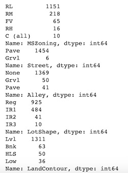
We are not dealing with features having high cardinality. Even if some features have low frequency categories, it may be worth keep them instead of grouping with other.

We can make the same analysis for ordinal features.

Since no issue arises, we can move to the encoding part, taking into account that a different approach is required for ordinal and nominal categorical features.

Also, it’s a good practice to typecast categorical features to a category dtype because they make the operations much faster than the object dtype. This can do by using the .astype() method on each columns like shown below:

df[nominal_features] = df[nominal_features].astype('category')

df[ordinal_features] = df[ordinal_features].astype('category')

We can check the current datatype by using the .dtypes() method

df[nominal_features].dtypes.head(3)

df[ordinal_features].dtypes.head(3)

Encoding Ordinal Features
When encoding ordinal features (the categories of which have an intrinsec order) we need to make sure that the learning algorithm takes into account the order of the categories. For that we have to map the categorical values to integer values manually.

We can use a dictionary-mapping approach along with the replace() function.

Note: Some of the ordinal features (‘OverallQual’,’OverallCond’, ‘YearBuilt’,’YearRemodAdd’,’MoSold’ and ‘YrSold’) do not need encoding since they are already in a numeric format.

For the other we proceed as shown below

mapping_dict = {
"ExterQual": {'Ex':4, 'Gd':3, 'TA':2, 'Fa':1},\
"ExterCond": {'Ex':4, 'Gd':3, 'TA':2, 'Fa':1},\
"BsmtQual":{'Ex':4, 'Gd':3, 'TA':2, 'Fa':1,'None':0},\
"BsmtCond":{'Gd':4, 'TA':3, 'Fa':2,'Po':1, 'None':0},\
"BsmtExposure":{'Av':4, 'Gd':3, 'Mn':2, 'No':1, 'None':0},\
"BsmtFinType1":{'GLQ':6,'ALQ':5, 'BLQ':4, 'Rec':3, 'LwQ':2,'Unf':1,'None':0},\
"BsmtFinType2":{'GLQ':6,'ALQ':5, 'BLQ':4, 'Rec':3, 'LwQ':2,'Unf':1,'None':0},\
"HeatingQC" :{'Ex':5, 'Gd':4, 'TA':3, 'Fa':2,'Po':1},\
"KitchenQual":{'Ex':4, 'Gd':3, 'TA':2, 'Fa':1},\
"GarageQual":{'Ex':5, 'Gd':4, 'TA':3, 'Fa':2,'Po':1,'None':0},\
"GarageCond":{'Ex':5, 'Gd':4, 'TA':3, 'Fa':2,'Po':1,'None':0},\
"Fence":{'GdPrv':4,'MnPrv':3, 'GdWo':2,'MnWw':1, 'No Fence':0}
}

df.replace(mapping_dict, inplace=True)

Encoding Nominal Features
To map nominal features (i.e. variables having multiple categories without any intrinsic ordering to them) we can use a technique called one-hot encoding. The idea behind this approach is to create a new dummy feature for each unique value in the nominal feature column.

Many libraries support one-hot encoding (e.g. sklearn), however the fastes way to do that is to use the pandas .get_dummies() method.

The most important arguments are

•   the DataFrame we want to encode on
  
•   the columns we want to do encoding on
  
•   the prefix argument which lets us specify the prefix for the new columns that will be created after encoding
  
•   the drop_first argument which, when set to True, leaves the first category of the feature out. This missing category becomes the the reference category for all further interpretation.
  This approach allows to avoid a risk of introduce into the regression redundant information, resulting in multicollinearity, and in a poor fit model.
  

nominal_features_dummies = pd.get_dummies(df[nominal_features], drop_first=True)

After creating our dummy variables, we concatenate them to the dataframe and we remove the original columns.

df = pd.concat([df, nominal_features_dummies], axis = 1)

df.drop(nominal_features, axis = 1, inplace = True)

df.drop(ordinal_features, axis = 1, inplace = True)

Scaling Features

This operation is needed when certain features in the dataset have a higher ‘magnitude’ than others.

In such cases, since most machine learning algorithms take into account only the magnitude of the measurements and not the units of those measurements, if no scaling is performed, features having high magnitude will have a much larger impact on the prediction than features having lower magnitude, regardless their actual relative importance.

Scaling features allows for features to contribute relative to their importance rather than their scale, by bringing all of them to an equivalent range of values.

Different approaches can be used to scale the features. The most commonly used and implemented in the Python ML package scikit-learn are :

• StandardScaler
• MinMaxScaler
• RobustScaler
• Normalizer

We use the RobustScaler which is robust to outliers.

Before scaling features, we need to split data into target (the value we want to predict, in this case the SalePrice) and features (all the columns the model uses to make a prediction). We have also to convert the dataframes to Numpy arrays in order to implement the model.

y_train = np.array(df['SalePrice'])
X_train = np.array(df.iloc[:,2:])

After that, we import the sklearn’s module for preprocessing, we create an object of the class ‘RobustScaler’ and we pass to it our train set as follows

from sklearn import preprocessing
scaler = preprocessing.RobustScaler()
X_train_scaled = scaler.fit_transform(X_train)

The next article, we’ll be focused on building a model to make prediction about home’s prices.